Performance Tips
Overview
This guide provides strategies to optimize performance when using GenericTensorNetworks.jl. We'll cover:
- Optimizing contraction orders
- Using slicing techniques for large problems
- Accelerating computations with specialized GEMM operations
- Leveraging multiprocessing for parallel execution
- Utilizing GPU acceleration
- Performance benchmarks and comparisons
1. Optimizing Contraction Orders
Let's examine how to optimize contraction orders using the independent set problem on 3-regular graphs:
using GenericTensorNetworks, Graphs, Random
graph = random_regular_graph(120, 3)
iset = IndependentSet(graph)
problem = GenericTensorNetwork(iset; optimizer=TreeSA(
    score=ScoreFunction(sc_target=20, sc_weight=1.0, rw_weight=3.0), ntrials=10, βs=0.01:0.1:15.0, niters=20))
The GenericTensorNetwork constructor maps a problem to a tensor network with an optimized contraction order. The optimizer parameter specifies the algorithm to use:
Available Optimizers:
- TreeSA (used above): A simulated annealing-based optimizer that often finds the smallest time/space complexity and supports slicing. See arXiv: 2108.05665 for details.
- GreedyMethod (default): Fastest search but typically yields higher contraction complexity
- KaHyParBipartite: Uses hypergraph partitioning
- SABipartite: Simulated annealing on bipartite representation
The returned problem object contains a code field specifying the tensor network with optimized contraction order. For an independent set problem, the optimal contraction complexity is approximately 2^(tw(G)), where tw(G) is the tree-width of graph G.
Analyzing Contraction Complexity
You can check the time, space, and read-write complexity with:
contraction_complexity(problem)This returns log2 values of:
- Number of multiplications
- Number of elements in the largest tensor during contraction
- Number of read-write operations to tensor elements
In our example, the computation requires approximately 2^21.9 multiplications, 2^20 read-write operations, and the largest tensor contains 2^17 elements.
Memory Requirements
Different element types have different memory footprints:
sizeof(TropicalF64)
sizeof(TropicalF32)
sizeof(StaticBitVector{200,4})
sizeof(TruncatedPoly{5,Float64,Float64})
For a more accurate estimate of peak memory usage in bytes, use:
estimate_memory(problem, GraphPolynomial(; method=:finitefield))
estimate_memory(problem, GraphPolynomial(; method=:polynomial))
The finite field approach requires only 298 KB, while using the Polynomial type requires 71 MB.
Note:
- Actual runtime memory can be several times larger than the maximum tensor size
- For mutable element types like
ConfigEnumerator, memory estimation functions may not accurately measure actual usage
2. Slicing Technique for Large Problems
For large-scale applications, you can slice over certain degrees of freedom to reduce space complexity. This approach loops and accumulates over selected degrees of freedom, resulting in smaller tensor networks inside the loop. This can be achieved by setting the slicer parameter of the GenericTensorNetwork constructor.
# Without slicing
problem = GenericTensorNetwork(iset; optimizer=TreeSA(βs=0.01:0.1:25.0, ntrials=10, niters=10))
contraction_complexity(problem)

# With slicing over 5 degrees of freedom
problem = GenericTensorNetwork(iset; optimizer=TreeSA(βs=0.01:0.1:25.0, ntrials=10, niters=10), slicer=TreeSASlicer(score=ScoreFunction(sc_target=10)))
contraction_complexity(problem)
In this example, slicing with the TreeSASlicer to reach space complexity of 2^10, at the cost of increased time complexity.
3. Accelerating Tropical Number Operations
You can significantly speed up Tropical number matrix multiplication when computing SizeMax() by using specialized GEMM routines from TropicalGEMM:
using BenchmarkTools

# Without TropicalGEMM
@btime solve(problem, SizeMax())
# 91.630 ms (19203 allocations: 23.72 MiB)
# 0-dimensional Array{TropicalF64, 0}:
# 53.0ₜ

# With TropicalGEMM
using TropicalGEMM
@btime solve(problem, SizeMax())
# 8.960 ms (18532 allocations: 17.01 MiB)
# 0-dimensional Array{TropicalF64, 0}:
# 53.0ₜ
TropicalGEMM overrides the LinearAlgebra.mul! interface and takes effect immediately upon loading. This example shows more than 10x speedup on a single-threaded CPU. Performance can be further improved with Julia multi-threading.
4. Multiprocessing for Parallel Execution
The GenericTensorNetworks.SimpleMultiprocessing submodule provides a convenient multiprocess_run function for parallel jobs. Here's how to find independence polynomials for multiple graphs using 4 processes:
# File: run.jl
using Distributed, GenericTensorNetworks.SimpleMultiprocessing
using Random, GenericTensorNetworks  # to avoid multi-precompilation
@everywhere using Random, GenericTensorNetworks

results = multiprocess_run(collect(1:10)) do seed
    Random.seed!(seed)
    n = 10
    @info "Graph size $n x $n, seed= $seed"
    g = random_diagonal_coupled_graph(n, n, 0.8)
    gp = GenericTensorNetwork(IndependentSet(g); optimizer=TreeSA())
    res = solve(gp, GraphPolynomial())[]
    return res
end

println(results)
Run this script with:
$ julia -p4 run.jl5. GPU Acceleration
To run computations on a GPU, simply load CUDA and set the usecuda parameter:
using CUDA
# [ Info: OMEinsum loaded the CUDA module successfully

solve(problem, SizeMax(), usecuda=true)
# 0-dimensional CuArray{TropicalF64, 0, CUDA.Mem.DeviceBuffer}:
# 53.0ₜ
GPU-Compatible Solution Properties:
SizeMaxandSizeMinCountingAllCountingMaxandCountingMinGraphPolynomialSingleConfigMaxandSingleConfigMin
6. Performance Benchmarks
We benchmarked performance on an Intel Xeon CPU E5-2686 v4 @ 2.30GHz (single thread) and a Tesla V100-SXM2 16GB GPU. The benchmark code is available in our paper repository.
Independent Set Problem Benchmarks
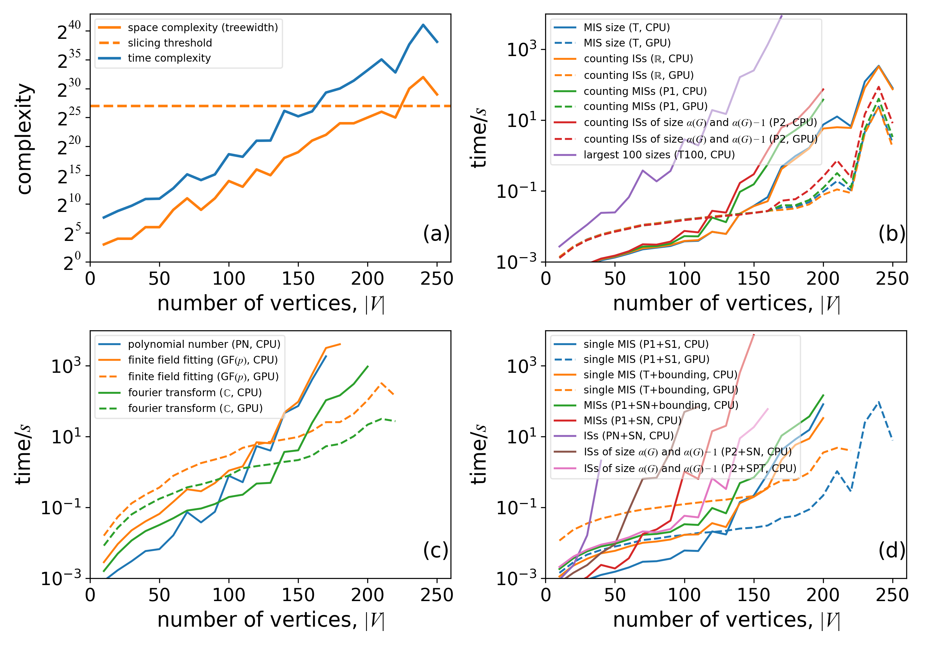
These benchmarks show computation time for various independent set properties on random three-regular graphs:
Figure (a): Time and space complexity vs. number of vertices
- Slicing was used for graphs with space complexity > 2^27 (above yellow line)
Figure (b): Computation time for:
- MIS size calculation
- Counting all independent sets
- Counting MISs
- Counting sets of size α(G) and α(G)-1
- Finding 100 largest set sizes
Figure (c): Computation time for independence polynomials:
- Fourier transformation method is fastest but may have round-off errors
- Finite field (GF(p)) approach has no round-off errors and works on GPU
Figure (d): Configuration enumeration time:
- Bounding techniques improve performance by >10x for MIS enumeration
- Bounding also significantly reduces memory usage
Maximal Independent Set Benchmarks
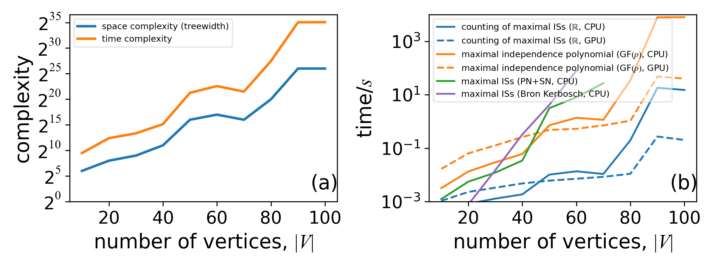
Figure (a): Time and space complexity for maximal IS problems
- Typically higher than for standard independent set problems
Figure (b): Wall clock time comparison:
- Counting maximal ISs is much more efficient than enumeration
- Our tensor network approach is slightly faster than Bron-Kerbosch for enumerating maximal ISs