Tsim

A fast sampler for noisy quantum circuits with non-Clifford gates, built on the ZX-calculus. Tsim feels just like Stim, but supports T gates, arbitrary rotations, and other non-Clifford instructions.

A detailed description of Tsim is given in arXiv:2604.01059.

Quick Start

An introductory tutorial is available here. For many existing scripts, replacing stim with tsim should just work. Tsim mirrors the Stim API and supports all Stim instructions, plus the non-Clifford instructions listed below.

import tsim

c = tsim.Circuit(
    """
    RX 0
    R 1
    T 0
    PAULI_CHANNEL_1(0.1, 0.1, 0.2) 0 1
    H 0
    CNOT 0 1
    DEPOLARIZE2(0.01) 0 1
    M 0 1
    DETECTOR rec[-1] rec[-2]
    """
)

detector_sampler = c.compile_detector_sampler()
samples = detector_sampler.sample(shots=100)

Installation

uv add bloqade-tsim

The default sampling strategy runs on the CPU. To run the stabilizer-rank strategies on an NVIDIA GPU, install the JAX CUDA extra:

uv add "bloqade-tsim[cuda13]"

See Installation for more options.

Sampling Strategies

Tsim offers two ways to simulate the non-Clifford parts of a circuit. Both start from the same ZX diagram. Choose a strategy with the strategy argument of compile_sampler and compile_detector_sampler.

sampler = c.compile_detector_sampler(strategy="cat5")

The stabilizer rank strategies are provisional; see API stability.

The Tsim 1.0 blog post introduces the active state vector strategy and compares its performance with other simulators.

Architecture

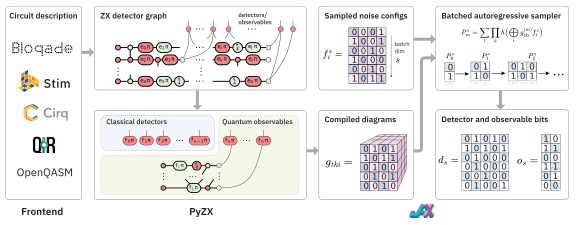
Quantum programs are translated into ZX diagrams in which Pauli noise channels appear as parameterized vertices with binary variables \(e_i\). ZX simplification factors the diagram into a classical part that represents the Tanner graph and a quantum part containing the observable circuit. Both parts define a new basis of error mechanisms \(f_i = \bigoplus_j T_{ij}\,e_j\). Outputs that depend on the error mechanisms alone are sampled directly from the noise model. The remaining components of the observable diagram are simulated in one of two ways:

• Active state vector. Each component is read off the reduced ZX diagram, without circuit extraction, as a sequence of Pauli rotations and measurements on \(|0\dots0\rangle\). Tsim then simulates it on a dense state vector over its active qubits, an approach that follows Clifft (Chase and Labib, 2026) and SymFT (Fang, Lou and Li, 2026).
• Stabilizer rank. Each component is decomposed into a sum of Clifford terms, following Sutcliffe and Kissinger (2024), and compiled into binary JAX tensors \(g_{tki}\). JIT-compiled XLA kernels contract \(g_{tki}\) with batched noise configurations \(f_i^{s}\) to evaluate marginal probabilities and autoregressively sample detector and observable bits.

Differences from Stim

Tsim supports non-deterministic detectors and observables. An important consequence is that Tsim will simulate actual detector samples, whereas Stim only reports detection flips (i.e. detection samples XORed with a noiseless reference sample). Concretely,

c = tsim.Circuit(
    """
    X 0
    M 0
    DETECTOR rec[-1]
    """
)
sampler = c.compile_detector_sampler()
samples = sampler.sample(shots=100)
print(samples)

samples = sampler.sample(
    shots=100,
    use_detector_reference_sample=True,
    use_observable_reference_sample=True,
)

Supported Instructions

Tsim supports all Stim instructions. In addition, Tsim defines the following non-Clifford instructions. Angles are given in units of π (half-turns).

T 0 1 2                  # T on qubits 0, 1, 2
R_Z(0.125) 2             # rotate qubit 2 around Z by π/8
U3(0.5, 0.25, 0.125) 0   # θ=π/2, φ=π/4, λ=π/8
TPP X0*Y1                # exp(-i π/8 · X0⊗Y1)
R_ZZ(0.5) 0 2            # exp(-i π/4 · Z0⊗Z2)
R_PAULI(0.3) X0*Y1*Z2    # exp(-i 0.3·π/2 · X0⊗Y1⊗Z2)
CCX 0 1 2                # Toffoli with controls 0, 1 and target 2

Postselected simulations

For postselected QEC experiments, pass a boolean mask to CompiledDetectorSampler.sample. The mask has length num_detectors; a shot is discarded when any masked detector fires, and only the other shots are returned.

import numpy as np

c = tsim.Circuit(
    """
    X_ERROR(0.01) 0 1
    M 0 1
    DETECTOR rec[-2]
    DETECTOR rec[-1] rec[-2]
    OBSERVABLE_INCLUDE(0) rec[-1]
    """
)
sampler = c.compile_detector_sampler()
mask = np.array([True, False])  # postselect on detector 0

shots = 10_000
survivors = sampler.sample(
    shots=shots,
    postselection_mask=mask,
    append_observables=True,
)
acceptance_rate = len(survivors) / shots

With a mask, sample returns at most shots rows, possibly none; without one, exactly shots rows. With separate_observables, both arrays hold the same shots. Shots discarded by a direct postselected detector (one that is a single error bit or a constant) skip the remaining component sampling. With strategy="active_statevector", a shot discarded by a component detector also stops being simulated, while stabilizer-rank components are computed in full.

The mask tests the values that sample returns: with use_detector_reference_sample, a shot is kept when its masked detectors match the noiseless reference sample, and otherwise when their raw parities are 0. A masked detector that is a constant 1, such as one of a noiseless circuit whose measurements have parity 1, discards every shot; sample warns about it.

API stability

Tsim follows semantic versioning for its public API: tsim.Circuit, tsim.CompiledMeasurementSampler and tsim.CompiledDetectorSampler. tsim.experimental holds helpers that may change in any release. Every other module is internal, even where it is importable. The stabilizer rank sampling strategies ("cat5", "bss", "cutting") are provisional: they may be removed in a minor release, after at least one minor release in which they emit a DeprecationWarning. See the API reference.

A seed reproduces its samples only with the same versions of Tsim and its dependencies (such as NumPy and JAX) and the same backend (CPU or GPU). With a stabilizer-rank strategy, pass the same explicit batch_size as well, since the default batch size depends on the free memory.

Citing Tsim

If you use Tsim, please consider citing the paper describing the core simulation approach:

@article{tsim2026,
  title={Tsim: Fast Universal Simulator for Quantum Error Correction},
  author={Haenel, Rafael and Luo, Xiuzhe and Zhao, Chen},
  journal={arXiv preprint arXiv:2604.01059},
  year={2026}
}

You may also cite the work by Sutcliffe and Kissinger (2024):

@article{sutcliffe2024fast,
  title={Fast classical simulation of quantum circuits via parametric rewriting in the ZX-calculus},
  author={Sutcliffe, Matthew and Kissinger, Aleks},
  journal={arXiv preprint arXiv:2403.06777},
  year={2024}
}

The active state vector strategy builds on Clifft and SymFT:

@article{chase2026clifft,
  title={Clifft: Fast Exact Simulation of Near-Clifford Quantum Circuits},
  author={Chase, Bradley A. and Labib, Farrokh},
  journal={arXiv preprint arXiv:2604.27058},
  year={2026}
}

@article{fang2026symft,
  title={SymFT: Universal Fault-Tolerant Quantum Circuit Simulation via Symbolic Clifford--Pauli Frames and Stabilizer Coordinates},
  author={Fang, Wang and Lou, Huazhe and Li, Riling},
  journal={arXiv preprint arXiv:2607.28600},
  year={2026}
}