Hamiltonian in a 3-level system

The Hamiltonian in a 3-level system is similar to a 2-level system. It also consists of Rabi terms, detuning terms, and Rydberg interaction between atoms but with more levels. The convention we used for a 3-level system Hamiltonian is

\[i \hbar \dfrac{\partial}{\partial t} | \psi \rangle = \hat{\mathcal{H}}(t) | \psi \rangle, \\ \begin{aligned} \frac{\mathcal{H}(t)}{\hbar} = & \sum_i \frac{\Omega_i^{\mathrm{hf}}(t)}{2}\left(e^{i \phi_i^{\mathrm{hf}}(t)}|0_i\rangle\langle 1_i|+e^{-i \phi_i^{\mathrm{hf}}(t)}| 1_i\rangle\langle 0_i|\right)-\sum_i \Delta_i^{\mathrm{hf}}(t)|1_i\rangle\langle 1_i| \\ & +\sum_i \frac{\Omega_i^{\mathrm{r}}(t)}{2}\left(e^{i \phi_i^{\mathrm{r}}(t)}|1_i\rangle\langle r_i|+e^{-i \phi_i^{\mathrm{r}}(t)}| r_i\rangle\langle 1_i|\right)-\sum_i\left[\Delta_i^{\mathrm{hf}}(t)+\Delta_i^{\mathrm{r}}(t)\right]\left|r_i\right\rangle\left\langle r_i\right| \\ & +\sum_{i<j} V_{i j}\left|r_i\right\rangle\left\langle r_i|\otimes| r_j\right\rangle\left\langle r_j\right| . \end{aligned}\]

Here, $|0\rangle$ and $|1\rangle$ represent two different hyperfine levels in a atom. And $|r\rangle$ represent the Rydberg level we use for entangling different atoms. There are two seperated pulses: the first one couples two hyperfine levels $|0\rangle$ and $|1\rangle$ and the second couples the hyperfine level $|1\rangle$ and the Rydberg level $|r\rangle$. We use two different superscripts $\mathrm{hf}$ and $\mathrm{r}$ to indicate them respectively.

Interface for the 3-level Hamiltonian

The interface for defining a 3-level Rydberg Hamiltonian is rydberg_h_3. It is similar as the 2-level interface rydberg_h. The only difference is that, in 3-level you need to specify the Rabi term $(\Omega, \phi)$ and the detunning term $(\Delta)$ for both hyperfine coupling $(\Omega^{\mathrm{hf}}, \phi^{\mathrm{hf}}, \Delta^{\mathrm{hf}})$ and rydberg coupling $(\Omega^{\mathrm{r}}, \phi^{\mathrm{r}}, \Delta^{\mathrm{r}})$. And both time-dependent and site-dependent waveforms are supported for each parameter (see Hamiltonians for details about defining different waveforms).

Pulse sequences and quantum gates

We can use two hyperfine levels to represent a qubit. In this case single-qubit gates can be directly obtained using hyperfine coupling in the 3-level system, and two-qubit gates can also be implemented by the coupling between $|1\rangle$ and $|r\rangle$ with the assist of Rydberg interation between different Rydberg atoms. In general, any n-qubit unitary can be approximated by a 3-level Rydberg pulse sequence. Hence, the 3-level Rydberg system is universal for qubit quantum computation.

Single-qubit gates

Here is an example for applying a Pauli $X$ gate (acting on hyperfine levels $|0\rangle$ and $|1\rangle$) to each site. Notes that single qubit gates could be parallelize, that is implementing the same single qubit gate on different sites with only one pulse.

julia> using Bloqade
julia> atoms = generate_sites(ChainLattice(), 5, scale=5)5-element AtomList{1, Float64}:
 (0.0,)
 (5.0,)
 (10.0,)
 (15.0,)
 (20.0,)
julia> h = rydberg_h_3(atoms; Ω_hf = 1.0)nqudits: 5
+
├─ [+] ∑ 2π ⋅ 8.627e5.0/|x_i-x_j|^6 n^r_i n^r_j
└─ [+] 2π ⋅ 0.0796 ⋅ ∑ σ^{x,hf}_i
julia> reg = zero_state(5; nlevel = 3); # the initial state is an all-zero state
julia> prob = KrylovEvolution(reg, 0.0:1e-2:pi, h); # an X gate is a π-pulse
julia> emulate!(prob);
julia> measure(reg) # the final state is an all-one state1-element Vector{BitBasis.DitStr64{3, 5}}:
 11111 ₍₃₎

Two-qubit gates

Two-qubit gates can be implemented with the assist of Rydberg interaction between two atoms. Here we give two example of different implementation of the CZ-gate using the 3-level Rydberg system.

5-pulse CZ-gate
The Levine-Pichler gate

Notes that the gate set of arbitrary single-qubit gate + CZ-gate is universal. Hence, 3-level Rydberg system is universal for quantum computing.

5-pulse CZ-gate

Suppose we have two atoms which are cloesed to each other so that there is Rydberg blockade between them. And the first atom is the controlling qubit while the second atom is the target qubit.

julia> using Bloqade
julia> atoms = generate_sites(ChainLattice(), 2; scale = 4)2-element AtomList{1, Float64}:
 (0.0,)
 (4.0,)

There are 5 steps in total for the CZ-gate.

Apply an X-gate (hyperfine π-pulse) on each qubit to flip $|0\rangle$ and $|1\rangle$
Apply an Rydberg π-pulse on the controlling qubit
Apply an Rydberg 2π-pulse on the target qubit
Apply an Rydberg π-pulse on the controlling qubit
Apply an X-gate (hyperfine π-pulse) on each qubit to flip $|0\rangle$ and $|1\rangle$

To understand the above steps, let us consider two different cases when the controlling qubit starts with $|0\rangle$ and $|1\rangle$.

If the controlling qubit starts with $|0\rangle$, then after step 2 it will be

excited into the Rydberg state $|r\rangle$. Because of the Rydberg blockade, the pulse in step 3 act trivially but a global phase -1 onto the target qubit. This means nothing changes but a global phase -1 if controlling qubit is $|0\rangle$.

If the controlling qubit is started with $|1\rangle$, then after step 2 it will

become the hyperfine state $|0\rangle$ which will not affect the pulse in step 3. In this case, the 2π-pulse will cause a phase -1 only if the target qubit is $|1\rangle$ after step 2 (which means the target qubit starts with $|0\rangle$). This means a Z-gate upto a global phase -1 is applied on the target qubit when the controlling qubit is $|1\rangle$.

The following codes implement the above 5-steps of the CZ-gate.

julia> using Bloqade
julia> using Yao
julia> atoms = generate_sites(ChainLattice(), 2; scale = 4)2-element AtomList{1, Float64}:
 (0.0,)
 (4.0,)
julia> st = zeros(ComplexF64, 9); st[[1, 2, 4, 5]] .= 1/2; # [1, 2, 4, 5] are indices for hyperfine states
julia> reg = arrayreg(st; nlevel = 3)  # initialize the state with 1/2 (|00⟩ + |01⟩ + |10⟩ + |11⟩)ArrayReg{3, ComplexF64, Array...}
    active qudits: 2/2
    nlevel: 3
julia> hs = [
           rydberg_h_3(atoms; Ω_hf = [1.0, 1.0]),  # hyperfine pulse for step 1
           rydberg_h_3(atoms; Ω_r = [1.0, 0.0]),   # Rydberg pulse for step 2
           rydberg_h_3(atoms; Ω_r = [0.0, 1.0]),   # Rydberg pulse for step 3
           rydberg_h_3(atoms; Ω_r = [1.0, 0.0]),   # Rydberg pulse for step 4
           rydberg_h_3(atoms; Ω_hf = [1.0, 1.0]),  # hyperfine pulse for step 5
       ]   # Hamiltonians for step 1-55-element Vector{RydbergHamiltonian3}:
 nqudits: 2
+
├─ [+] ∑ 2π ⋅ 8.627e5.0/|x_i-x_j|^6 n^r_i n^r_j
└─ [+] ∑ Ω_i ⋅ σ^{x,hf}_i

 nqudits: 2
+
├─ [+] ∑ 2π ⋅ 8.627e5.0/|x_i-x_j|^6 n^r_i n^r_j
└─ [+] ∑ Ω_i ⋅ σ^{x,r}_i

 nqudits: 2
+
├─ [+] ∑ 2π ⋅ 8.627e5.0/|x_i-x_j|^6 n^r_i n^r_j
└─ [+] ∑ Ω_i ⋅ σ^{x,r}_i

 nqudits: 2
+
├─ [+] ∑ 2π ⋅ 8.627e5.0/|x_i-x_j|^6 n^r_i n^r_j
└─ [+] ∑ Ω_i ⋅ σ^{x,r}_i

 nqudits: 2
+
├─ [+] ∑ 2π ⋅ 8.627e5.0/|x_i-x_j|^6 n^r_i n^r_j
└─ [+] ∑ Ω_i ⋅ σ^{x,hf}_i
julia> ts = [π, π, 2π, π, π]   # pulse time for step 1-55-element Vector{Float64}:
 3.141592653589793
 3.141592653589793
 6.283185307179586
 3.141592653589793
 3.141592653589793
julia> step = 1e-3; # Krylov time step
julia> for i = 1:5
           prob = KrylovEvolution(reg, 0.0:step:ts[i], hs[i])
           emulate!(prob)
       end
julia> state(reg)[1, 2, 4, 5]  # equivalent to 1/2 (|00⟩ + |01⟩ + |10⟩ - |11⟩)ERROR: BoundsError: attempt to access 9×1 Matrix{ComplexF64} at index [1, 2, 4, 5]

The Levine-Pichler gate

A more efficient way to implementing the CZ-gate is using the Levine-Pichler gate. Comparing to the above 5-pulse CZ-gate, the Levine-Pichler gate uses shorter sequence and less time.

Consider two atoms which are closed to each other. If we apply a pulse that couples $|1\rangle$ and $|r\rangle$ with the Rabi frequency $\Omega^\mathrm{r}$, detunning $\Delta^\mathrm{r}$, and duration $\tau$, then the dynamics of four hyperfine state are different.

$|00\rangle$ will not change during the pulse
$|01\rangle$ ($|10\rangle$) will oscillate between $|01\rangle$ and $|0r\rangle$ ($|10\rangle$ and $|r0\rangle$) with a frequency $\Omega^\mathrm{r}$
$|11\rangle$ will oscillate between $|11\rangle$ and $|w\rangle = \frac{1}{2}\left( |1r\rangle + |r1\rangle \right)$ with a frequency $\sqrt{2}\Omega^\mathrm{r}$ (this is an approximation when the Rydberg blockade is strong enough such that the population of $|rr\rangle$ could be ignored)

The Levine-Pichler gate consists of two global pulses. Together with a global hyperfine pulse for rotation-Z gates, we will get a CZ-gate.

A global Rydberg pulse with parameters $\frac{\Delta^\mathrm{r}}{\Omega^\mathrm{r}} \approx 0.377371$, $\phi^\mathrm{r} = 0$, $\Omega^\mathrm{r}\tau \approx 4.29268$
A global Rydberg pulse with parameters $\frac{\Delta^\mathrm{r}}{\Omega^\mathrm{r}} \approx 0.377371$, $\phi^\mathrm{r} \approx 3.90242$, $\Omega^\mathrm{r}\tau \approx 4.29268$
A global hyperfine pulse with parameters $\Delta^\mathrm{r}\tau = 2\pi - \alpha \approx 3.90242$, $\Omega^\mathrm{r} = \phi^\mathrm{r} = 0$

The first pulse completes a full cycle of oscillation for $|11\rangle$ while it does not complete a cycle for $|01\rangle$ and $|10\rangle$. The only difference between the first and the second pulse is the parameter $\phi^\mathrm{r}$. This difference causes a change of the rotation axis on the Bloch sphere, such that the second pulse completes another full cycle of oscillation for $|11\rangle$ while it also brings back $|01\rangle$ and $|10\rangle$. After these two pulses has a unitary representation

\[\begin{pmatrix} 1 & & & \\ & e^{i\alpha} & & \\ & & e^{i\alpha} & \\ & & & e^{i(2\alpha-\pi)} \end{pmatrix},\]

which is a CZ-gate with single qubit rotation gates $R_Z(\alpha)$ on each qubit. The following picture (Fig 2 c) in the original paper) demonstrates the process of the first pulse and the second pulse.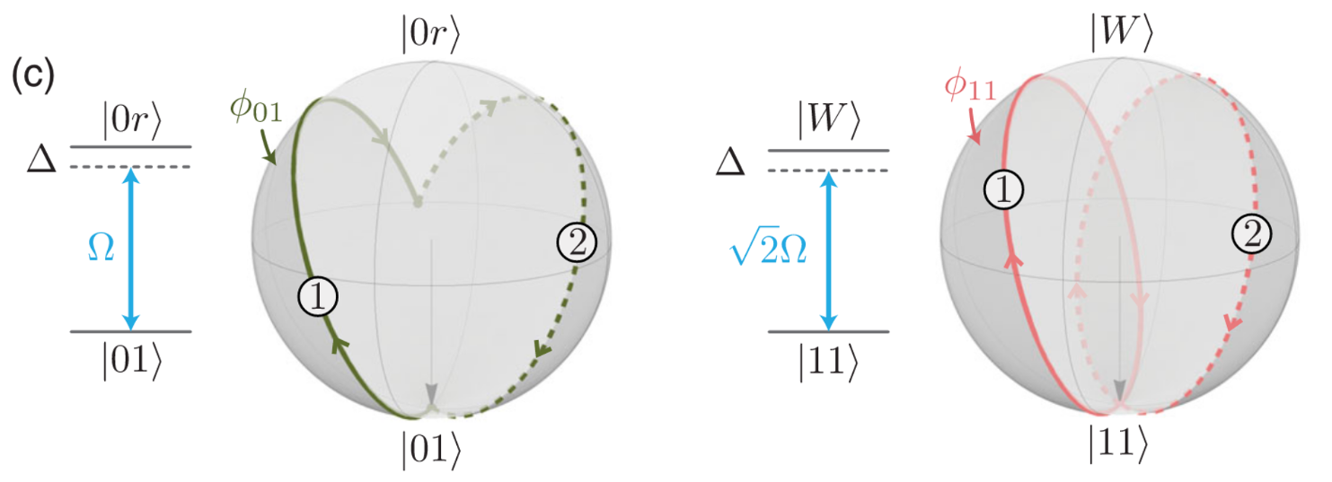

Here are codes for the Levine-Pichler gate.

julia> using Bloqade
julia> using Yao
julia> st = zeros(ComplexF64, 9); st[[1, 2, 4, 5]] .= 1/2; # [1, 2, 4, 5] are indices for hyperfine states
julia> reg = arrayreg(st; nlevel = 3); # initialize the state with 1/2 (|00⟩ + |01⟩ + |10⟩ + |11⟩)
julia> atoms = generate_sites(ChainLattice(), 2; scale = 4);
julia> Ω_r = 1.0; ϕ_r = 3.90242; Δ_r = 0.377371*Ω_r;   # define parameters
julia> τ = 4.29268/Ω_r; α = 2.38076;   # define pulse durations
julia> step = 1e-3;    # Krylov step
julia> hs = [
           rydberg_h_3(atoms; Ω_r = Ω_r, Δ_r = Δ_r),   # global Rydberg pulse for step 1
           rydberg_h_3(atoms; Ω_r = Ω_r, ϕ_r = ϕ_r, Δ_r = Δ_r),    # global Rydberg pulse for step 2
           rydberg_h_3(atoms; Δ_hf = 1.0), # global hyperfine pulse for R_Z-gate in step 3
       ]3-element Vector{RydbergHamiltonian3}:
 nqudits: 2
+
├─ [+] ∑ 2π ⋅ 8.627e5.0/|x_i-x_j|^6 n^r_i n^r_j
├─ [+] 2π ⋅ 0.0796 ⋅ ∑ σ^{x,r}_i
└─ [-] 2π ⋅ 0.0601 ⋅ ∑ n^r_i

 nqudits: 2
+
├─ [+] ∑ 2π ⋅ 8.627e5.0/|x_i-x_j|^6 n^r_i n^r_j
├─ [+] 2π ⋅ 0.0796 ⋅ ∑ e^{3.9 ⋅ im} |1⟩⟨r| + e^{-3.9 ⋅ im} |r⟩⟨1|
└─ [-] 2π ⋅ 0.0601 ⋅ ∑ n^r_i

 nqudits: 2
+
├─ [+] ∑ 2π ⋅ 8.627e5.0/|x_i-x_j|^6 n^r_i n^r_j
├─ [-] ∑ n^{hf}_i
└─ [-] ∑ n^r_i
julia> ts = [τ, τ, 2π - α]3-element Vector{Float64}:
 4.29268
 4.29268
 3.9024253071795862
julia> for i = 1:3 # simulation
           prob = KrylovEvolution(reg, 0:step:ts[i], hs[i])
           emulate!(prob)
       end
julia> state(reg)[[1, 2, 4, 5]]  # desired state 1/2 (|00⟩ + |01⟩ + |10⟩ - |11⟩)4-element Vector{ComplexF64}:
  0.5000000000000753 - 2.94757364114856e-16im
 0.49999993904048046 - 0.0002116027322570296im
 0.49999993904048046 - 0.0002116027322570296im
  -0.499999876854552 - 0.00033513730510956413im

Predefined pulse sequences for different quantum gates

Instead of defining pulse sequences manually, we provide lots of predefined pulse sequences for basic quantum gates. For more details, please refer to the package BloqadeGates.

References

The 3-level Rydberg Hamiltonian:

BloqadeExpr.rydberg_h_3 — Function

rydberg_h_3(atoms; [C=2π * 862690 * MHz*µm^6, 
    Ω_hf = nothing, ϕ_hf = nothing, Δ_hf = nothing, 
    Ω_r = nothing, ϕ_r = nothing, Δ_r = nothing])

Create a 3-level Rydberg Hamiltonian

\[\sum_{i<j} \frac{C}{|x_i - x_j|^6} n^r_i n^r_j + \sum_{i} \left[\frac{Ω^{\mathrm{hf}}}{2} (e^{iϕ^\mathrm{hf}}|0⟩⟨1| + e^{-iϕ^\mathrm{hf}}|1⟩⟨0|) - Δ^{\mathrm{hf}} n^{1}_i + \frac{Ω^{\mathrm{r}}}{2} (e^{iϕ^\mathrm{r}}|1⟩⟨r| + e^{-iϕ^\mathrm{r}}|r⟩⟨1|) - (Δ^{\mathrm{hf}} + Δ^{\mathrm{r}}) n^{\mathrm{r}}_i \right]\]

shorthand for

RydInteract(C, atoms; nlevel = 3) + 
    SumOfXPhase_01(length(atoms), Ω_hf/2, ϕ_hf) - SumOfN(length(atoms), Δ_hf) +
    SumOfXPhase_1r(length(atoms), Ω_r/2, ϕ_r) - SumOfN(length(atoms), Δ_r + Δ_hf)