Waveforms

Waveforms are essential ingredients for generating the Rydberg Hamiltonian. By controlling the waveforms of $\Omega$, $\Delta$, and $\phi$, one can prepare the ground states of certain target Hamiltonians and study their non-equilibrium dynamics. Bloqade supports several built-in waveforms and allows the users to specify waveforms by inputting functions. It also supports different operations of waveforms, such as waveform smoothening, composing, and more.

The generated waveforms can be directly used to build the time-dependent Hamiltonians. Please see the Hamiltonians section for more details.

Creating Waveforms

In Bloqade, the waveforms are defined as a Waveform object, which is a created by providing a callable object and a real number duration:

Bloqade gives users the flexibility to specify general waveforms by inputting functions. The following code constructs a sinusoidal waveform with a time duration of 2 μs:

using Bloqade
using PythonCall
plt = pyimport("matplotlib.pyplot")
waveform = Waveform(t->2.2*2π*sin(2π*t), duration = 2);
Bloqade.plot(waveform)

In our documentation, we use the python package matplotlib for plotting.

Bloqade supports built-in waveforms for convenience (see References below). For example, the codes below create different waveform shapes with a single line:

waveform = piecewise_linear(clocks=[0.0, 0.2, 0.5, 0.8, 1.0], values= 2π* [0.0, 1.5, 3.1, 3.1, 0.0]);
Bloqade.plot(waveform)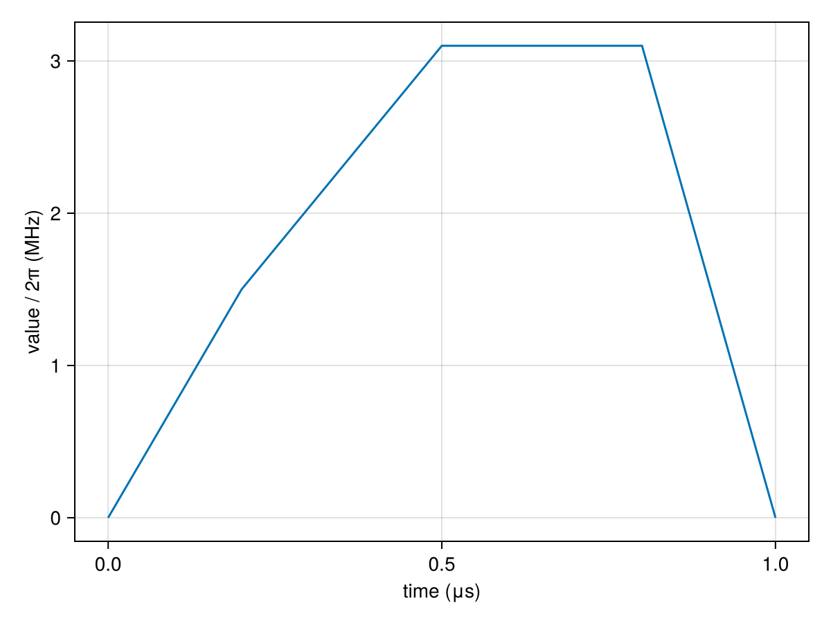

waveform = piecewise_constant(clocks=[0.0, 0.2, 0.5, 0.7], values= 2π*[0.0, 1.5, 3.1]);
Bloqade.plot(waveform)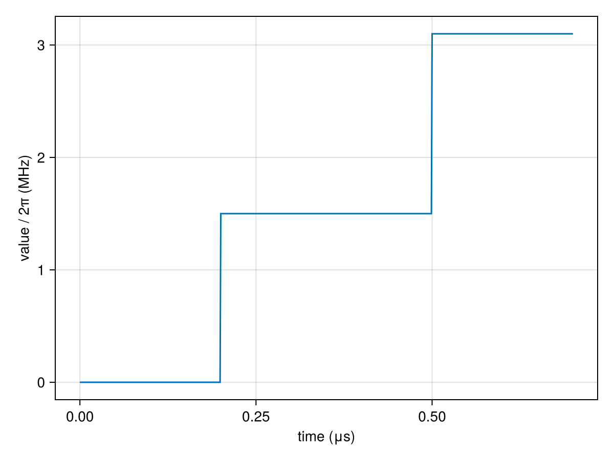

waveform = linear_ramp(duration=0.5, start_value=0.0, stop_value=2π*1.0);
Bloqade.plot(waveform)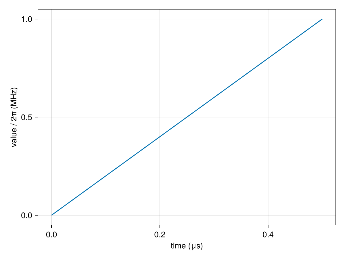

waveform =  constant(duration=0.5, value=2π*2.1);
Bloqade.plot(waveform)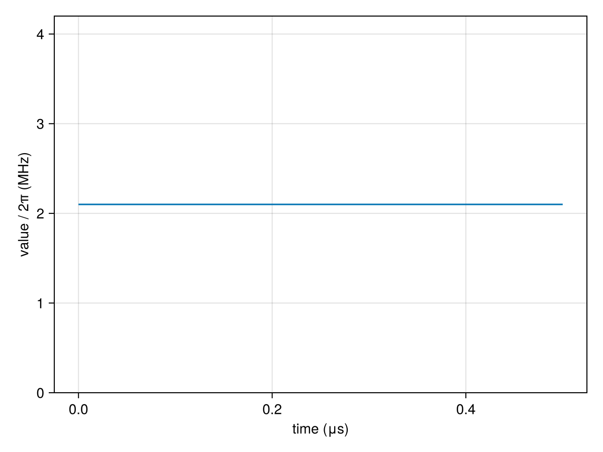

waveform = sinusoidal(duration=2, amplitude=2π*2.2);
Bloqade.plot(waveform)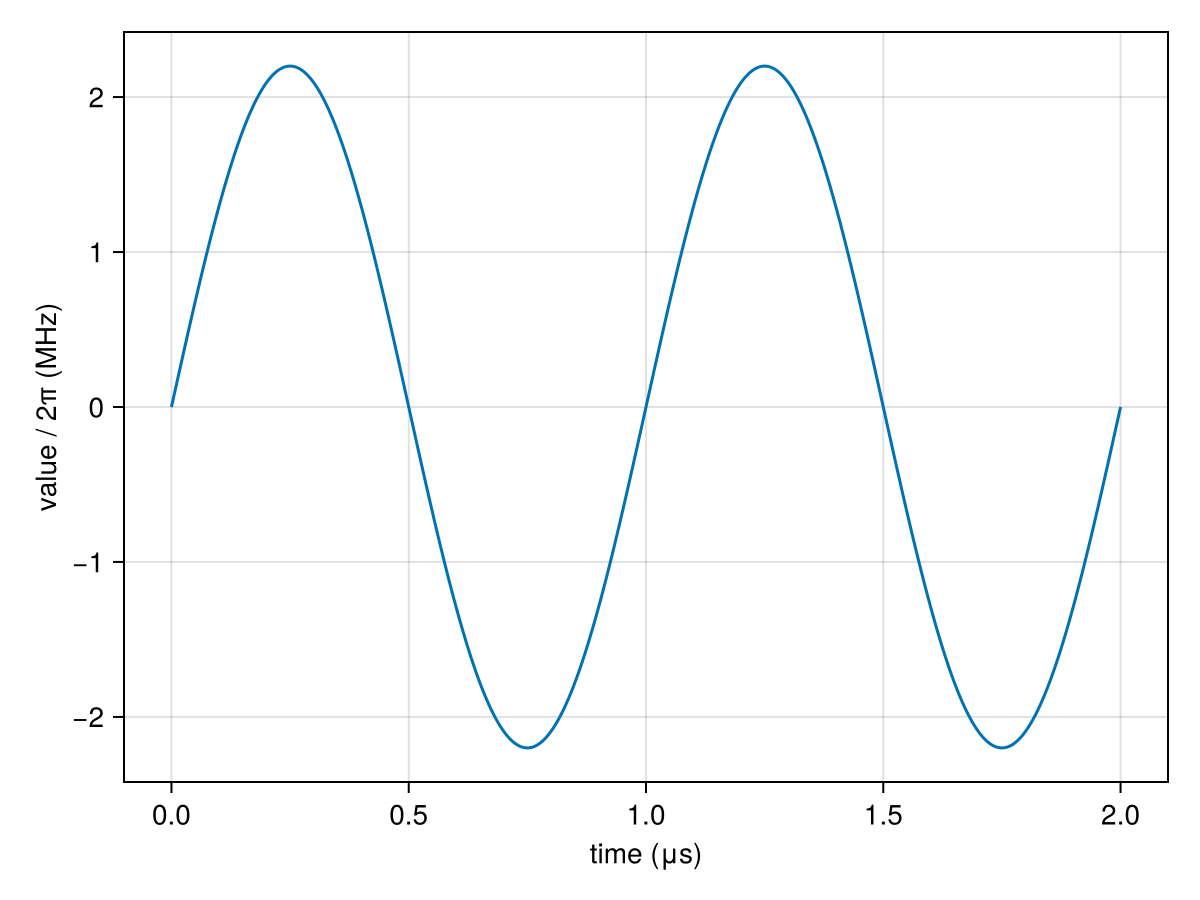

In some cases, users may have their own waveforms specified by a vector of clocks and a vector of signal strengths. To build a waveform from the two vectors, we can directly use the functions piecewise_linear or piecewise_constant, corresponding to different interpolations.

clocks = collect(0:1e-1:2);
values1 = 2π*rand(length(clocks));
wf1 = piecewise_linear(;clocks, values=values1);
values2 = 2π*rand(length(clocks)-1)
wf2 = piecewise_constant(;clocks, values=values2);

fig, (ax1, ax2) = plt.subplots(figsize=(12, 4), ncols=2)
Bloqade.plot!(ax1, wf1)
Bloqade.plot!(ax2, wf2)
fig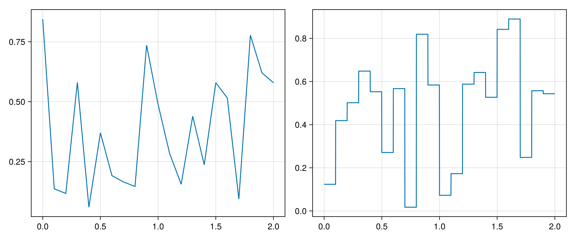

For more advanced interpolation options, please see the JuliaMath/Interpolations package.

Operations on Waveforms

Bloqade also supports several operations on the waveforms.

Waveforms can be sliced using the duration syntax start..stop, e.g.:

wf = 2π*sinusoidal(duration=2.2);
wf1 = wf[1.1..1.5];
Bloqade.plot(wf1)

Note that time starts from 0.0 again, so the total duration is stop - start.

Waveforms can be composed together via append:

wf2 = linear_ramp(;start_value=0.0, stop_value=1.1*2π, duration=0.5);
waveform = append(wf1, wf2);
Bloqade.plot(waveform)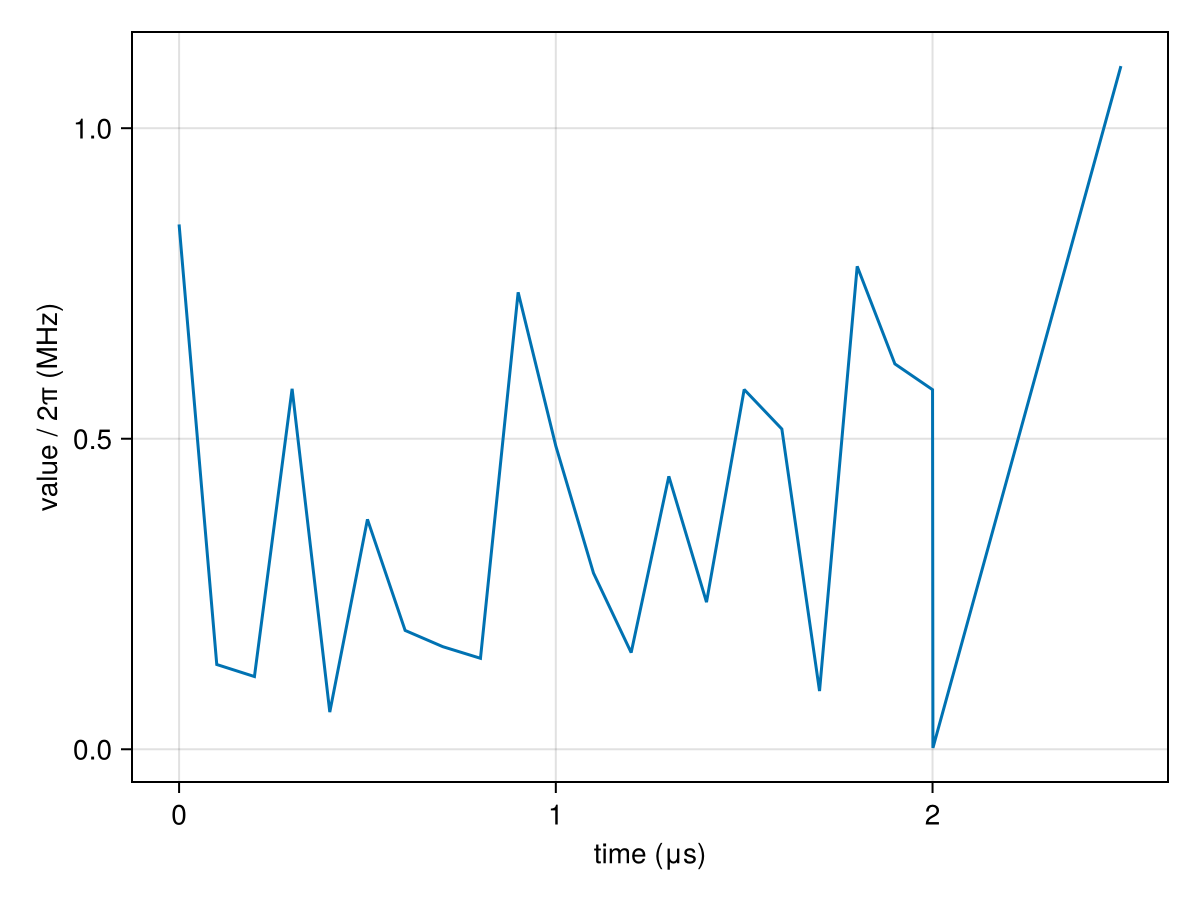

where the waveform wf2 is appended at the end of wf1.

Sharp points in waveforms may result in bad performance in practice (e.g. for adiabatically preparing a ground state of a target Hamiltonian). It is sometimes preferred to smoothen the waveform using the moving average methods. One can use the smooth function to create a smoothened waveform from a piecewise linear waveform:

wf = piecewise_linear(clocks=[0.0, 2.0, 3.0, 4.0], values=2π*[0.0, 3.0, 1.1, 2.2]);
swf = smooth(wf;kernel_radius=0.1);

fig, (ax1, ax2) = plt.subplots(figsize=(12, 4), ncols=2)
Bloqade.plot!(ax1, wf)
Bloqade.plot!(ax2, swf)
fig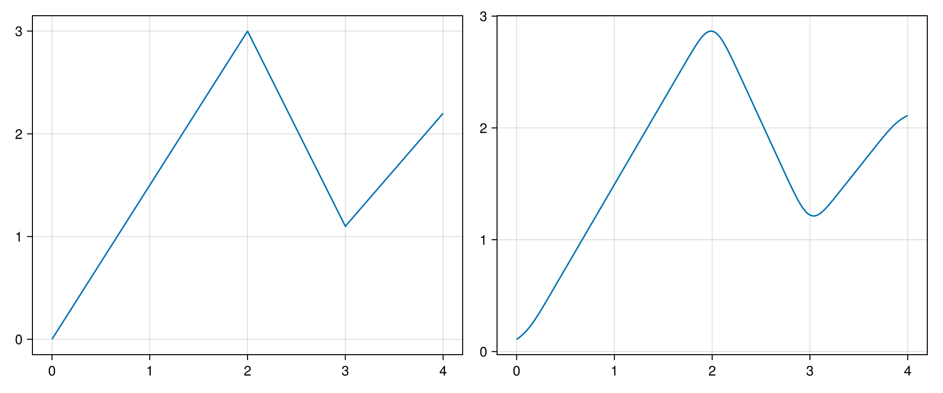

Waveform Arithmetics

Bloqade also supports several arithmetics on the waveforms. If two waveforms have the same duration, we can directly add up or subtract the strength of them, simply by using + or -:

wf1 = linear_ramp(;duration=2.2, start_value=0.0, stop_value=1.0*2π);
wf2 = sinusoidal(duration = 2.2, amplitude = 2.2*2π);
wf3 = wf1 + wf2;
wf4 = wf1 - wf2;

fig, (ax1, ax2) = plt.subplots(figsize=(12, 4), ncols=2)
Bloqade.plot!(ax1, wf3)
Bloqade.plot!(ax2, wf4)
fig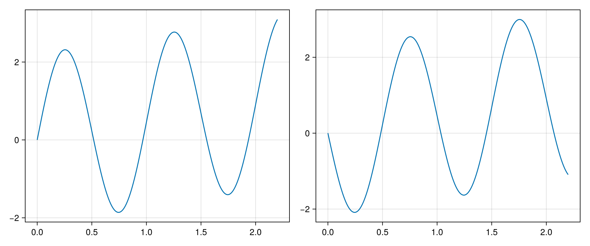

To increase the strength of a waveform by some factors, we can directly use *:

wf = linear_ramp(;duration=2.2, start_value=0.0, stop_value=1.0*2π);
wf_t = 3 * wf;

fig, (ax1, ax2) = plt.subplots(figsize=(12, 4), ncols=2)
Bloqade.plot!(ax1, wf)
Bloqade.plot!(ax2, wf_t)
fig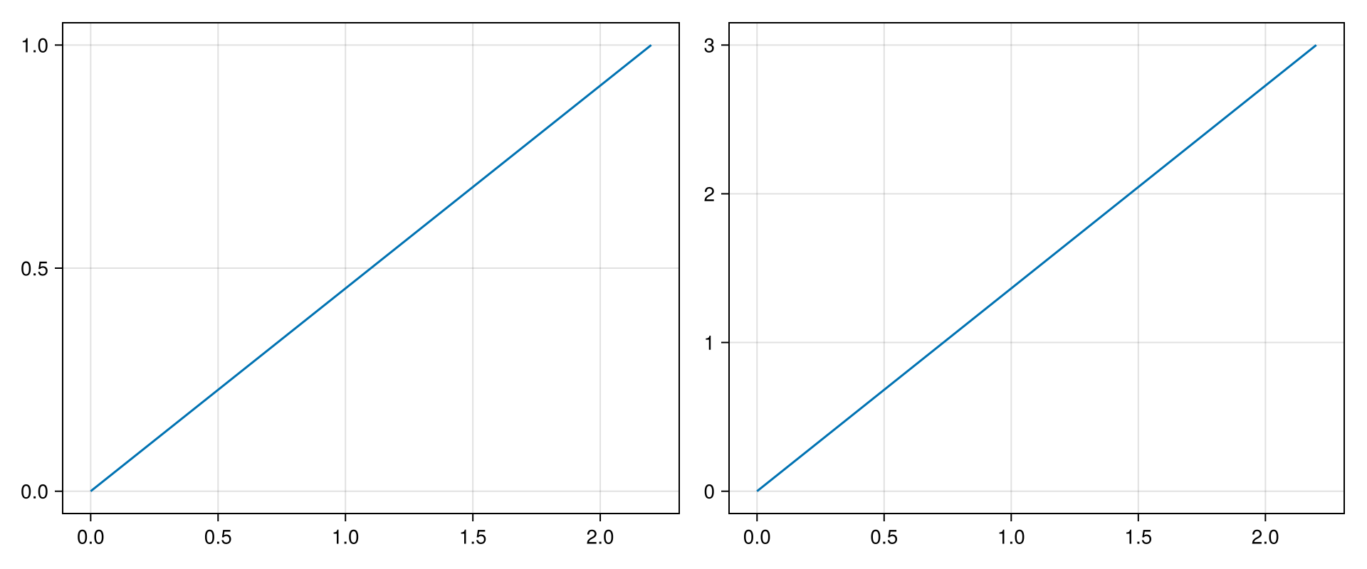

Such operations can also be broadcasted by using .*:

wf2, wf3 = [2.0, 3.0] .* wf1;

fig, (ax1, ax2) = plt.subplots(figsize=(12, 4), ncols=2)
Bloqade.plot!(ax1, wf2)
Bloqade.plot!(ax2, wf3)
fig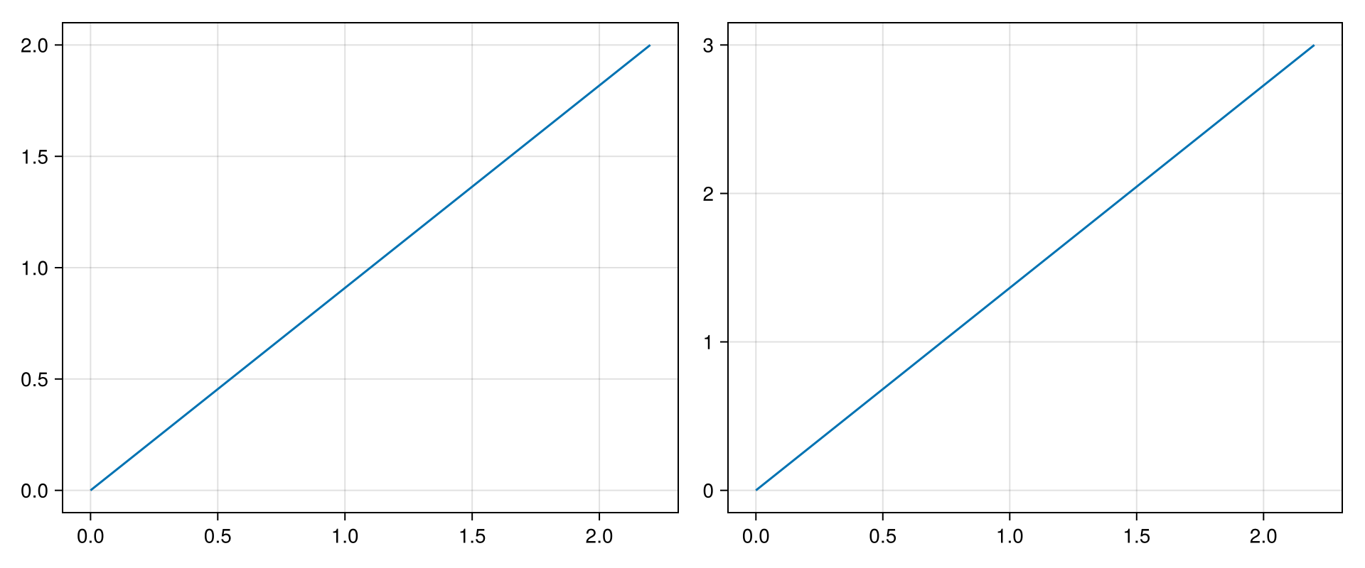

References

BloqadeWaveforms.Waveform — Type

struct Waveform{F,T<:Real}

Type for waveforms. Waveforms are defined as a function combined with a real number duration.

Fields

f: a callable object.
duration: a real number defines the duration of this waveform; default unit is μs.