Quantum Monte Carlo Method
In previous tutorials such as the Adiabatic Evolution one, Exact Diagonalization (ED) was used to produce the results. While ED is numerically exact and works for smaller systems consisting of tens of atoms it scales poorly. An alternative method that Bloqade supports is Quantum Monte Carlo (QMC) under the BloqadeQMC module which can scale to hundreds of atoms with the caveat that it is exact up to statistical errors.
It is worth clarifying that despite the name, QMC is a purely classical method that uses the Monte Carlo (MC) approach towards problems in quantum physics. To provide more context, the space we are generating samples from is a Hilbert space of quantum-mechanical configurations. Furthermore, QMC is one of the best established methods in numerically tackling the analytically intractable integrals of quantum many-body physics that are beyond the reach of exact solutions.
Background
Typically, the integral or sum in question is the expectation value of some observable $\langle A \rangle_\psi = \sum_j a_j |\langle \psi | \phi_j \rangle |^2$ such as the energy, magnetization etc. The issue we face is the curse of dimensionality, meaning the number of terms in this sum grows exponentially in system size. We circumvent this curse by not calculating the whole sum, but instead sampling from the probability distribution given by $|\langle \psi | \phi_j \rangle |^2$, favoring those terms that contribute significantly to the sum, i.e. have large weights $a_j$. While doing so, it is essential that we explore the configuration space ergodically. This means that configurations with a small but non-zero weight should have a chance of being reached, even though this will occur less frequently than for those with large weights.
While QMC is an umbrella term comprising many different implementations of this same core idea tailored to a specific class of quantum problems, BloqadeQMC currently implements the SSE (Stochastic Series Expansion) by Anders Sandvik, recently adapted for the Rydberg Hamiltonian by E. Merali et al (10.48550/arXiv.2107.00766).
Getting Started with BloqadeQMC
We begin by importing the required libraries:
using BloqadeQMC
using Random
In addition, we will import some libraries that can be used later to check our QMC against ED results for small system sizes:
using Bloqade, Bloqade.CairoMakie
using Yao: mat, ArrayReg
using LinearAlgebra
using Measurements
using Measurements: value, uncertainty
using Statistics
As an initial example, we recreate the hamiltonian for the $\mathbb{Z}_2$ phase in the 1D chain which we saw in the Adiabatic Evolution tutorial.
nsites = 9
atoms = generate_sites(ChainLattice(), nsites, scale = 5.72)

Ω = 2π * 4
Δ = 2π * 10
h = rydberg_h(atoms; Δ, Ω)
nqubits: 9
+
├─ [+] ∑ 2π ⋅ 8.627e5.0/|x_i-x_j|^6 n_i n_j
├─ [+] 2π ⋅ 2.0 ⋅ ∑ σ^x_i
└─ [-] 2π ⋅ 10.0 ⋅ ∑ n_i
Now we differ from the adiabatic evolution tutorial by passing the hamiltonian to rydberg_qmc:
h_qmc = rydberg_qmc(h);The object h_qmc still contains all the previous information about the lattice geometry as well as the Hamiltonian parameters $\Omega$ and $\Delta$. However, the object now also stores the distribution of weights from which the algorithm will sample. Without going into all the details which can be found in E. Merali et al (10.48550/arXiv.2107.00766), we can focus on those key elements of the SSE formalism that you will need to calculate observables from the samples. This requires understanding what is meant by configuration space in the SSE formalism, what samples from that space look like and what their weights are.
Prelude: Massaging the Partition Function
Before answering those questions, let us revisit the finite temperature partition function $Z = Tr(e^{-\beta H})$. Indeed, $Z$ is the protagonist in the mathematical formalism of SSE. Massaging it through a few tricks and combinatorics will help us answer the questions and prepare us for the diagram below.
The core idea is the following: Instead of calculating the trace analytically, we can first write out the Taylor series of the exponential:
\[Z = Tr(e^{-\beta H}) = Tr(\sum_{n=0}^{\infty} \frac{\beta^n}{n!}(-\hat{H})^n)\]
next, we insert the usual identities over a set of basis states $\{\alpha_p\}$, giving:
\[Z = \sum_{\{\alpha_p\}} \sum_{n=0}^{\infty}\frac{\beta^n}{n!} \prod_{p=1}^n \langle\alpha_{p-1}| -\hat{H} | \alpha_p\rangle\]
Finally, we split the Hamiltonian into a sum of local Hamiltonians where each term acts on only one or two atoms. (For example, the latter includes the Rydberg interaction term.) Formally, we will write $H = - \sum_{t, a} \hat{H}_{t,a}$ where the labels $t$ symbolizes whether the term is diagonal ($t=1$) or off-diagonal ($t=-1$) and $a$ specifies the atoms the term acts on. This leads to the last crucial step in massaging the partition function: We switch the order of the n-fold product and sum. From each copy of the total Hamiltonian, we pick one of the local terms and multiply these in a new n-fold product:
\[Z = \sum_{\{\alpha_p\}} \sum_{n=0}^{\infty} \sum_{S_n} \frac{\beta^n}{n!} \prod_{p=1}^n \langle\alpha_{p-1}| - \hat{H}_{t_p, a_p} | \alpha_p\rangle\]
For further technical details, please refer to Section 2.1 of E. Merali et al (10.48550/arXiv.2107.00766)
Why is this crucial? This procedure of picking local terms produced something we will refer to as an operator sequence and denote by $S_n$ with $n$ being the length of this sequence. We investigate what this looks like in the section below.
The SSE Configuration Space
Let us consider a system consisting of four Rydberg atoms. One state in the SSE configuration space of this system could look like the following:
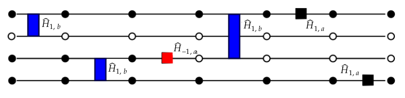
We define each element of the diagram above as follows:
- The four circles correspond to four atoms, with filled circles being excited atoms $|r\rangle$ and white circles representing the ground state $|g\rangle$.
- The blue, red and black boxes situated either on one horizontal line or sitting between two lines stand for the local Hamiltonian terms we mentioned earlier. The interested reader may find the full definition of the local terms in Section 3 of E. Merali et al (10.48550/arXiv.2107.00766)
- The seven copies of four atoms/six boxes are the the visual equivalent of looking at the sixth expansion order in the Taylor series introduced above. Each SSE sample will correspond to a particular expansion order $m$ since the infinite Taylor series gave rise to an intractable sum which we can use the core idea of MC to sample from.
Putting the pieces together, we should be able to understand the general idea of the weight distribution stored in the rydberg_qmc object. That distribution is given by the matrix elements defined by the local operators (boxes) sandwiched in between two configurations of the physical system (two copies of the four vertically stacked atoms). The picture as a whole is what defines one sample in the SSE configuration whose overall weight is given by the product of the matrix elements of each operator.
It is worth stating at this point that a precise understanding is not necessary to successfully run a simulation using BloqadeQMC. We have included this peek into the backend in order for the reader to have some notion of what we mean when we refer to the number of operators sampled in the energy calculations later on (equivalent to the number of boxes in the diagram above).
Running a Simulation using BloqadeQMC
Now that we have defined the configuration space, let us traverse it and generate samples from it. It is worth pointing out that the samples generated are no longer random and independent as they are in traditional MC but rely on Markov Chain Monte Carlo (MCMC). In MCMC, the samples are no longer independent but form a chain in which the probability of the next sample depends on the current sample.
Before jumping into the code, let us touch on the prototypical example of how such a chain might be built: via the Metropolis-Hastings algorithm. This recipe has three main steps:
Randomly propose a new configuration,
accept the proposal according to a probability given by the ratio of the weights of the current and proposed configuration,
\[P = min(\frac{W_{current}}{W_{proposed}}, 1)\]
- and repeat.
Now, let us define the parameters than govern the length of the chain, i.e. how long we let the simulation run for:
EQ_MCS = 100;
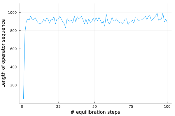
MCS = 100_000;Note that two parameters are required. MCMC simulation is typically split into two phases: first the equilibration phase, also referred to as the burn-in, followed by the sampling phase. While the mathematical theorems surrounding Markov Chains guarantee under reasonable assumptions these chains eventually converge to the desired probability distribution, it does take some time until this is the case.
While there is no formula that will tell you when precisely equilibration has been reached, a good heuristic is plotting an observable such as the energy. You will see its value initially fluctuate but stabilize around a value which you can then assume is its equilibrium expectation value.
Now, we are almost ready to run the simulation.
M = 50;
ts = BinaryThermalState(h_qmc, M);
BinaryThermalState is an object necessary in the backend to store the instantaneous SSE configuration during the MC steps.
d = Diagnostics();Diagnostics are a feature that can be used by the advanced user to analyse performance and extract further information from the backend.
Next, we choose the inverse temperature β to be large enough for the simulation to approximate the ground state. If your system is gapped, then a finite value for β will be enough to reach the ground state. If the gap closes, then you will need to scale β with the system size.
β = 0.5;

rng = MersenneTwister(3214);
Finally, we initialize the pseudorandom number generator. We can now execute the simulation.
Note that mc_step_beta! returns three objects which can be used for computations during each MC step. ts stores the instantaneous SSE configuration, h_qmc is the same object as before, lsize is related to the arrays used to carry out a MC step and depend on the operator sequence of the current configuration.
Furthermore, SSE_slice stores a sample of the atom configuration taken from the current SSE configuration, in this case chosen to be the first vertical slice.
[mc_step_beta!(rng, ts, h_qmc,β, d, eq=true) for i in 1:EQ_MCS] # equilibration phase

densities_QMC = zeros(nsites)
occs = zeros(MCS, nsites)

for i in 1:MCS # Monte Carlo Steps
    mc_step_beta!(rng, ts, h_qmc,β, d, eq=false) do lsize, ts, h_qmc
        SSE_slice = sample(h_qmc,ts, 1)
        occs[i, :] = ifelse.(SSE_slice .== true, 1.0, 0.0)
    end
end

for jj in 1:nsites
    densities_QMC[jj] = mean(occs[:,jj])
end
Let us plot the results.
fig = Figure()
ax = Axis(fig[1, 1]; xlabel="Site number", ylabel="Occupation density")
results_plot = barplot!(ax, densities_QMC)
results_plot
MakieCore.Plot{Makie.barplot, Tuple{Vector{GeometryBasics.Point{2, Float64}}}}As expected, we see a $\mathbb{Z}_2$ pattern has emerged, just as we saw using the exact diagonalization method. So let us try an example that goes beyond what is feasible with ED.
We run the same code as before, substituting the 1D chain with 9 atoms for a 2D square lattice with 100 atoms.
nx = ny = 10;
nsites = nx*ny;
atoms = generate_sites(SquareLattice(), nx, ny, scale = 6.51);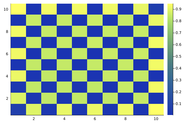
Calculating Observables using BloqadeQMC
The final question we will address in this tutorial is how to calculate observables using BloqadeQMC. We will choose to investigate the energy during a detuning sweep. Furthermore, we will limit ourselves to a system size which ED can also handle such that we may compare the results from both methods.
Let us start by returning to the 1D chain and defining the Hamiltonian parameters. We will keep the constant Rabi drive from before, i.e. $\Omega = 2\pi \times 4$ MHz. For the detuning, we will choose the following ramp.
nsites = 9;
atoms = generate_sites(ChainLattice(), nsites, scale = 5.72);

Δ_step = 15;
Δ = LinRange(-2π * 9, 2π * 9, Δ_step);
Now, we only need to make two small changes to our previous MC code. First, for each value of $\Delta$ specified in this ramp, we will run a separate QMC simulation that will produce one data point in the final energy plot. Second, we need to store the number of operators contained in each sample. Yes, this is where the picture we introduced earlier comes in. This number will fluctuate from sample to sample as we build the Markov chain. It is directly returned by the mc_step_beta!() function.
We can then use the number of operators to compute the energy due to the following observation. Firstly, we know from statistical physics that:
\[\langle E \rangle = -\frac{\partial ln Z}{\partial \beta}\]
Yet in the SSE formalism we can find another expression for the expectation value $\langle E \rangle$. Let us work backwards and consider the SSE expectation value of the length of the operator sequence:
\[\begin{aligned} \langle n \rangle &= \frac{1}{Z} Tr(\sum_{n=0}^\infty n \frac{(-\beta \hat{H})^n}{n!}) \\ &= \frac{1}{Z} Tr(\sum_{n=1}^\infty n \frac{(-\beta \hat{H})^n}{n!}) \\ &= \frac{1}{Z} Tr(\sum_{n=1}^\infty \frac{(-\beta \hat{H})^n}{(n-1)!}) \\ &= \frac{1}{Z} Tr(\sum_{n=0}^\infty (-\beta \hat{H}) * \frac{(-\beta \hat{H})^n}{n!}) \end{aligned}\]
where in the second line we dropped the vanishing $n=0$ term and in the fourth line we shifted the sum over n by 1 and obtained the extra factor $-\beta \hat{H}$. From this, we directly read of the SSE formula for the energy expectation value:
\[\langle E \rangle = -\frac{\langle n \rangle}{\beta}\]
using BinningAnalysis

energy_QMC = []

for ii in 1:Δ_step
    h_ii = rydberg_h(atoms; Δ = Δ[ii], Ω)
    h_ii_qmc = rydberg_qmc(h_ii)
    ts_ii = BinaryThermalState(h_ii_qmc,M)
    d_ii = Diagnostics()

    [mc_step_beta!(rng, ts_ii, h_ii_qmc, β, d_ii, eq=true) for i in 1:EQ_MCS] #equilibration phase

    ns = zeros(MCS)

    for i in 1:MCS # Monte Carlo Steps
        ns[i] = mc_step_beta!(rng, ts_ii, h_ii_qmc, β, d_ii, eq=false)
    end

    energy(x) = -x / β + h_ii_qmc.energy_shift  # The energy shift here ensures that all matrix elements are non-negative. See Merali et al for details.
    BE = LogBinner(energy.(ns)) # Binning analysis
    τ_energy = tau(BE)
    ratio = 2 * τ_energy + 1
    energy_binned = measurement(mean(BE), std_error(BE)*sqrt(ratio))
    append!(energy_QMC, energy_binned)
end
There is one last point worth addressing when calculating expectation values using a MCMC method. As mentioned previously, the samples are not statistically independent, instead they are correlated due to the Markov Chain property. This point is crucial. After all, Monte Carlo is exact only in a statistical sense. We must construct error bars around the mean values generated by our simulation. The correlation of samples has the effect of reducing the effective variance, thus purporting an accuracy we cannot in fact justify.
One method of addressing this issue is via binning analysis. The idea is to bin small sequences of samples together and average over them. This gives rise to an reduced effective sample size given by:
\[N_{eff} = \frac{N_{orig}}{2\tau + 1}$\]
where $\tau$ is the autocorrelation time.
We use this effective sample size to rescale the standard error by $\sqrt{2\tau + 1}$. For details, please see the documentation of the BinningAnalysis package. If the error bars thus achieved are still too large, increasing the number of samples taken, i.e. the number of Monte Carlo steps can help alleviate the problem.
Finally, let us carry out the ED calculation as well and plot both results together.
energy_ED = zeros(Δ_step)

for ii in 1:Δ_step
    h_ii = rydberg_h(atoms; Δ = Δ[ii], Ω)
    h_m = Matrix(mat(h_ii))
    energies, vecs = LinearAlgebra.eigen(h_m)

    w = exp.(-β .* (energies .- energies[1]))
    energy_ED[ii] = sum(w .* energies) / sum(w)
end

fig = Figure()
ax = Axis(fig[1, 1]; xlabel="Δ/2π", ylabel="Energy")
scatter!(ax, Δ/2π, energy_ED, label="ED", marker=:x);
errorbars!(ax, Δ/2π, value.(energy_QMC), uncertainty.(energy_QMC))
scatter!(ax, Δ/2π, value.(energy_QMC); label="QMC", marker=:x)
axislegend(ax, position=:rt)
fig
We see that using the QMC, we have achieved the same results as for the ED with high accuracy.
As a final note, it is possible to also calculate other observables in the SSE formalism if they are products of the operators present in the Hamiltonian itself. For example, to calculate $\langle X \rangle$, one would count the number of times the off-diagonal operator $\sigma_x$ appears in each sample and take its average. For more examples and derivations, please see A. Sandvik (10.1088/0305-4470/25/13/017)*
To conclude this tutorial, we will leave with one final plot of the staggered magnetization which acts as an order parameter to observe the transition from the disordered to the $\mathbb{Z}_2$ phase achieved before:
densities_QMC = []
order_param_QMC = []

for ii in 1:Δ_step
    h_ii = rydberg_h(atoms; Δ = Δ[ii], Ω)
    h_ii_qmc = rydberg_qmc(h_ii)
    ts_ii = BinaryThermalState(h_ii_qmc,M)
    d_ii = Diagnostics()

    [mc_step_beta!(rng, ts_ii, h_ii_qmc, β, d_ii, eq=true) for i in 1:EQ_MCS] #equilibration phase

    order_param = zeros(MCS)

    for i in 1:MCS # Monte Carlo Steps
        mc_step_beta!(rng, ts_ii, h_ii_qmc, β, d_ii, eq=false) do lsize, ts_ii, h_ii_qmc
            SSE_slice = sample(h_ii_qmc, ts_ii, 1) # occ = 0,1
            spin = 2 .* SSE_slice .- 1 # spin = -1, 1
            order_param[i] = abs(sum(spin[1:2:end]) - sum(spin[2:2:end]))/length(spin)
        end
    end

    BD = LogBinner(order_param)
    τ_energy = tau(BD)
    ratio = 2 * τ_energy + 1
    energy_binned = measurement(mean(BD), std_error(BD)*sqrt(ratio))
    append!(order_param_QMC, measurement(mean(BD), std_error(BD)*sqrt(ratio)) )
end

fig = Figure()
ax = Axis(fig[1, 1]; xlabel="Δ/2π", ylabel="Stag mag")
errorbars!(ax, Δ/2π, value.(order_param_QMC), uncertainty.(order_param_QMC))
fig_order = scatter!(ax, Δ/2π, value.(order_param_QMC); label="", marker=:x)
axislegend(ax, position=:rt)
fig
This page was generated using Literate.jl.